Differentiating 1D Integrals #

by Shuang Zhao

In what follows, we discuss the differentiation of a simple Riemann integral $I(\theta)$ over some 1D interval $(a, b) \subseteq \real$:

The Incomplete Solution #

The derivative of the integral in Eq. \eqref{eqn:I} with respect to $\theta$ can sometimes be obtained by exchanging the ordering of differentiation and integration:

Precisely, the second equality in Eq. \eqref{eqn:dI_0} requires the integrand $f$ to be continuous¹ throughout the interval $(a, b)$.

Success Example #

We now provide a toy example where Eq. \eqref{eqn:dI_0} holds. Let $f(x, \theta) := x^2 \,\theta$. Consider the following integral:

Since $I = \left[ (x^3 \,\theta)/3 \right]_0^1 = \theta/3$, we know that

We now try calculating the same derivative $\D I/\D\theta$ using Eq. \eqref{eqn:dI_0}:

which matches the manually calculated result above.

Failure Example #

We now show another toy example for which simply exchanging differentiation and integration outlined in Eq. \eqref{eqn:dI_0} fails. Let

Then, for any $0 < \theta < 2$, it holds that

and

However, since the integrand $f$ is piecewise-constant in this example, we have $\D f/\D\theta \equiv 0$. Thus, Eq. \eqref{eqn:dI_0} in this example gives

which does not match the manually calculated result in Eq. \eqref{eqn:f_step_dI_manual}.

The General Solution #

Examining The Previous Examples #

Before presenting the general expression of the derivative $\D I/\D\theta$, we first examine the examples shown above.

The Success Example #

We first examine the success example with the integrand $f(x, \theta) = x^2 \,\theta$. In the following, we show the graph of $f(x, \theta)$ for some fixed $\theta = \theta_0$ in the following: 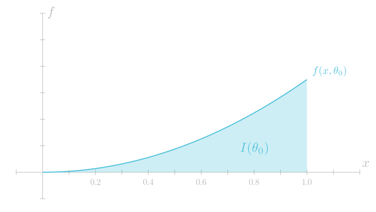By definition, the integral $I(\theta_0) := \int_0^1 f(x, \theta) \,\D x$ equals the signed area (marked in light blue) of the region below the graph. Further, by adding some small $\Delta\theta > 0$ to $\theta_0$, we obtain the graph of $f(x, \theta_0 + \Delta\theta)$ and the corresponding signed area $I(\theta_0 + \Delta\theta)$, both illustrated in red:

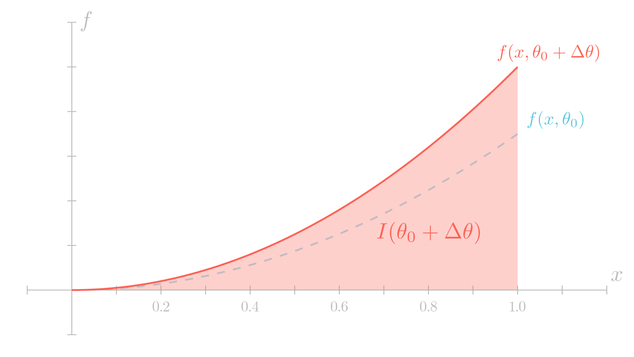
We recall that the derivative of $I$ with respect to $\theta$ is given by the rate at which $I$ changes with $\theta$. To calculate this rate, we examine the difference between $I(\theta_0 + \Delta\theta)$ and $I(\theta_0)$:

Geometrically, this difference equals the (signed) area of the orange region illustrated below:

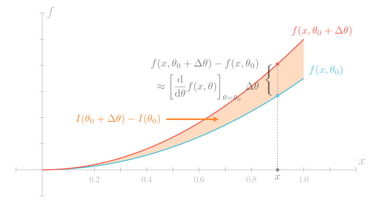
At each fixed $0 < x < 1$, the integrand of Eq. \eqref{eqn:diffI0_0} satisfies that

Base on this relation, we can rewrite the area difference \eqref{eqn:diffI0_0} as:

In both equations above, the equalities become exact at the limit of $\Delta\theta \to 0$. By dividing both sides by $\Delta\theta$ and taking the limit of $\Delta\theta \to 0$, we have

for any $0 < \theta_0 < 1$. This agrees with the incomplete solution expressed in Eq. \eqref{eqn:dI_0}.

The Failure Example #

So what has been the cause for the failure example? To be specific, what has been missing from the incomplete solution \eqref{eqn:dI_0}?

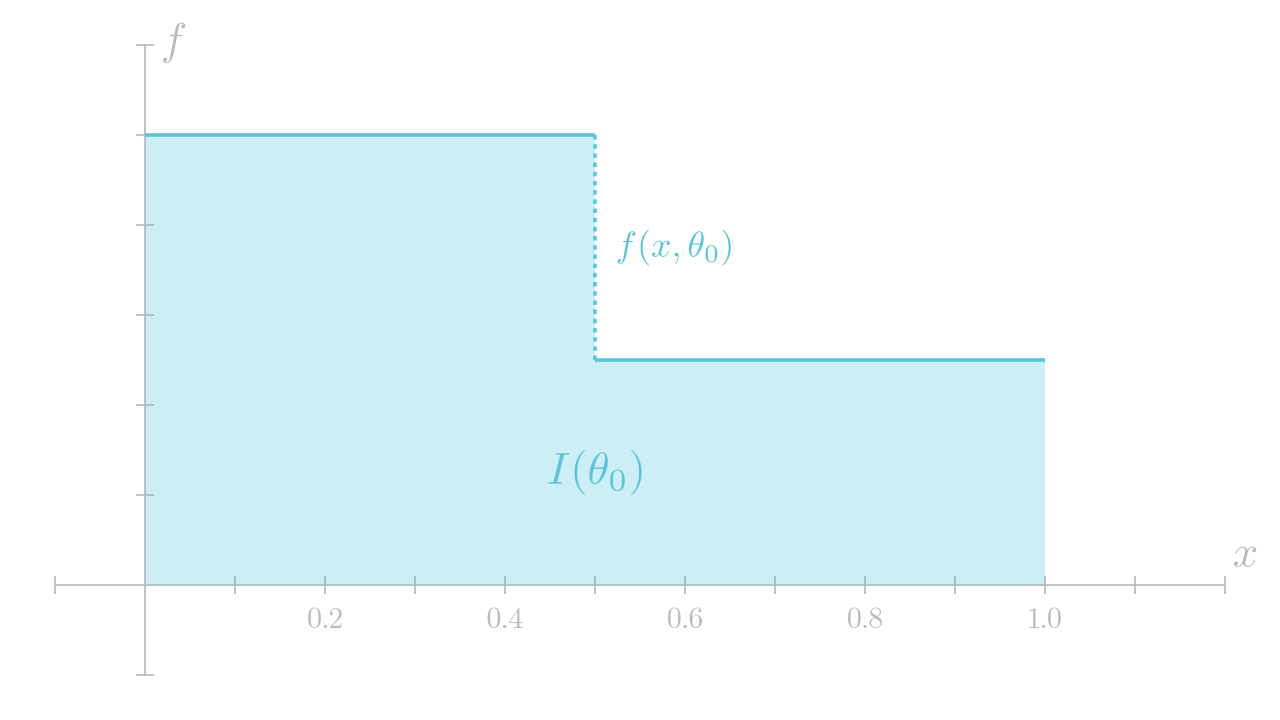
To understand what has been going on, we again examine the integrand $f(x, \theta)$ which, for this example, is the piecewise-constant function defined in Eq. \eqref{eqn:f_step}.

The following are the graphs of $f(x, \theta)$ for some fixed $\theta = \theta_0$ and $\theta = \theta_0 + \Delta\theta$ (for some small $\Delta\theta > 0$), respectively:

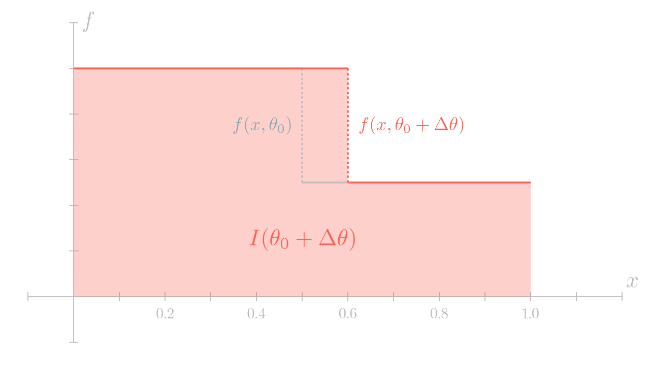
Further, the difference $I(\theta_0 + \Delta\theta) - I(\theta_0)$ between the signed areas below the two graphs is caused by the rectangle illustrated in orange:

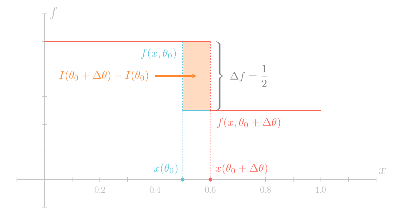
Intuitively, in the success example, the change of signed area is caused by vertical shifts of the graph—which is captured by the incomplete solution \eqref{eqn:dI0}. On the other hand, in this failure example, the change of signed area is caused by horizontal shifts of the graph _at jump discontinuities—which is missing from the incomplete solution!

We now calculate the signed area of the orange rectangle shown above. We first observe that the length of the rectangle’s vertical edge equals the difference $\Delta f \equiv 1 - 1/2 = 1/2$ of the integrand $f(x, \theta)$ across the discontinuity point.

To calculate the length of the rectangle’s horizontal edge, we let $x(\theta) = \theta/2$ denote the jump discontinuity point of $f(x, \theta)$ defined in Eq. \eqref{eqn:f_step}. Then, the (signed) length of the horizontal edge is simply $x(\theta_0 + \Delta\theta) - x(\theta_0)$.

Based on the observations above, we know that

Dividing both sides of this equation by $\Delta t$ and taking the limit $\Delta\theta \to 0$ produce:

Therefore, we know that

matching the hand-derived result in Eq. \eqref{eqn:f_step_dI_manual}.

The Full Derivative #

Based on the observations above, we now present the general derivative of the 1D integral expressed in Eq. \eqref{eqn:I}:

which comprises:

• A interior component obtained by exchanging differentiation and integration operations—identical to Eq. \eqref{eqn:dI_0}.

• A boundary component involving a sum over all jump discontinuity points $\{ x_i(\theta) : i = 1, 2, \ldots \}$.

Remarks #

Precisely, $\Delta f(x, \theta)$ in the boundary component is defined as

where $\lim_{u \uparrow x}$ and $\lim_{u \downarrow x}$ denote one-sided limits with $u$ approaching $x$ from below (i.e., $u < x$) and above (i.e., $u > x$), respectively. For any fixed $\theta$, $\Delta f(x, \theta)$ is nonzero (and well-defined) if and only if $x$ is a jump discontinuity point of $f(\cdot, \theta)$.

Lastly, when the endpoints $a$ and $b$ of the integral depend on $\theta$, they should be considered as jump discontinuities with $\Delta f(a, \theta) = -f(a, \theta)$ and $\Delta f(b, \theta) = f(b, \theta)$.

In the next section, we will present a generalization of Eq. \eqref{eqn:dI} that describes derivatives of Lebesgue integrals.